The scope of the Earth Observation Data Management System (EODMS) is to provide users the ability to search and download Level 1 products from a range of satellites to fulfill their information needs. The application of Level 1 products from SAR satellites typically requires the use of special processing software and a high degree of expertise. To ease the application of products from RADARSAT-2 and the RADARSAT Constellation Mission (RCM), the Canada Centre for Mapping and Earth Observation (CCMEO) developed the SAR Toolbox (ST). The ST is integrated within EODMS and allows users to select a variety of processing options. Because the ST operates in a semi-automated manner, its use does not require significant interaction or SAR know-how.

The products available from the ST have been selected through cross-department consultations and can be grouped as follows: Low-level, pre-processing products with a wide user base such as orthorectification, speckle filtering and more; Mid-level products such as polarimetric decompositions and others to enable broad use of RCM’s new Compact Polarimetric (CP) beam modes; and High level downstream products relating to land deformation (InSAR) and lake ice extent, which can inform the operations of the Government of Canada. The ST allows users to define, save and reuse custom processing sequences. EODMS will notify users once processing has completed and the resultant products are available for download.

The CCMEO ensures that the ST software and processing options are rigorous, scientifically sound, standardised, and well tested. However, CCMEO will not intervene in its operation by users nor will it assess the quality of the products that are delivered. In other words, CCMEO assumes that users will evaluate the quality of ST products and, in addition, have the ability to use the products correctly. Lastly, users should be aware that the ST may not process their product order in near-real time (e.g., within a few hours). Depending on user demand and data volumes, the ST will stage the generation and delivery of products over timeframes that may range from few minutes to several days.

The ST offers processing options in the following categories:

· Radiometry

· Ortho-rectification/Mosaic

· Filters

· Utilities

· Polarimetry

· Interferometry

· Lake Ice Extent (coming shortly)

Readers are referred to the product definition section at the end of this document for all details about the directory structure, naming convention, and metadata for all files included in the ST delivery package.

IMPORTANT: Please note the access to ST is restricted to Government of Canada users only.

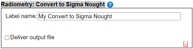
Radiometry

Radiometric Calibration

Quantitative analysis of SAR imagery requires that calibration be performed such that the image pixels values can be directly and accurately correlated with the backscatter values of the acquired scene. SAR data are typically made available to users as Level 1 products. Radiometric correction is necessary to correctly represent the backscatter from the surface observed. This also enables the quantitative analysis and comparison of images acquired at different times, by different sensors, or in different modes. The information necessary to calibrate SAR data is typically contained in the metadata and comes in the form of Look-Up Tables (LUTs). The EODMS SAR Toolbox offers calibration options. Depending on their preference, users can choose to have the data calibrated to beta-nought, sigma-nought, or gamma-nought values.

In the case of RCM ScanSAR products, all bursts are automatically merged to create one single image raster for each polarization.

Background electronic noise is not subtracted from the image product by default.

This method works for original (Level 1) input products only, i.e. CH, CV, HH, HV, VH, or VH.

The processing options are:

· Convert to Sigma Nought – The selected polarization(s) is calibrated to Sigma Nought values.

· Convert to Beta Nought - The selected polarization(s) is calibrated to Beta Nought values.

· Convert to Gamma Nought - The selected polarization(s) is calibrated to Gamma Nought values.

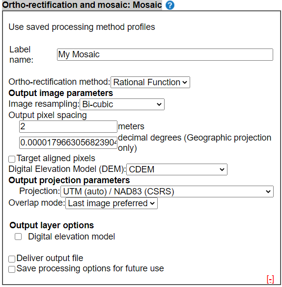
Ortho-rectification/Mosaic

Overview

Ortho-rectification is the process by which the effects of terrain and tilt are removed from an image. This process results in a planimetrically correct image, i.e. an image with coordinates that correctly ty to locations on the earth’s surface. As such, the image can be overlaid with other images, for the same area and in the same projection, and readily analyzed in a GIS. In short, the coordinates of pixels in the SAR image are transformed from the radar geometry to a map geometry—according to a projection selected by the user. Ortho-rectification of a SAR product requires information about the satellite’s orbit (contained in the product’s metadata) and an appropriate Digital Elevation Model (DEM). In the absence of a DEM, a fixed (average) elevation value can be used.

Rational Function

The Rational Function is a relatively simple math model that is used to develop a correlation between image pixels and corresponding ground locations for the precise geocoding of satellite imagery. Rational polynomial coefficients (RPC) are extracted from the image metadata and imported for use in the model. The polynomial coefficients are calculated from ground control points (GCPs) and combined with elevation data from a DEM to perform the ortho-rectification.

Constraints related to this method are:

· Only non-complex or detected products can be processed. The ST includes a utility to convert complex products to detected products.

This method works for original (Level 1) input products only, i.e. CH, CV, HH, HV, VH, or VH. Though, if by selecting “Process all selected Output layers from previous method(s)”, all output layers will also be ortho-rectified.

The following parameters must be specified:

Image resampling – Specify the resampling method to be applied to the image.

· Nearest Neighbour: nearest neighbor resampling assigns the output pixel the value of the nearest input pixel. It is the fastest resampling method available.

· Bi-linear: bi-linear resampling computes the value of the output pixel through two-dimensional cubic interpolation of the values of the 4 nearest input pixels.

· Bi-cubic: bi-cubic resampling computes the value of the output pixel through two-dimensional bi-cubic interpolation of the values of the 16 nearest input pixels.

Output pixel spacing - Specify a value for the output pixel spacing in meters or decimal degrees.

· meters;

· decimal degrees (Geographic projection only);

Target aligned pixels - align the coordinates of the extent of the output file to the values of the output pixel spacing, such that the aligned extent includes the minimum extent.

Digital Elevation Model (DEM). Select the preferred DEM to process the image.

· CDEM (Canada at 20m resolution)

· CDSM (CDEM+SRTM, Canada south of 60°N at 20m resolution)

· SRTM 30m (Canada south of 60°N at 30m resolution)

· SRTM 90m (World between 56°S and 60°N at 90m resolution)

· SRTM 30m (World between 56°S and 60°N at 30m resolution)

· ASTER 30m (World at 30m resolution)

Output Projection Parameters– Specify the desired output projection.

· UTM (auto) / NAD83 (CSRS)

· UTM (auto) / WGS84

· UTM / NAD83 (CSRS)

· UTM / WGS84

· Canada Atlas Lambert / NAD83 (EPSG:3978)

· Canada Albers Equal Area / NAD83 (EPSG:102001)

· Canada Crop Inventory Albers Equal Area / WGS84

· NSIDC Sea Ice Polar Stereographic North / WGS84 (EPSG:3413)

· NSIDC EASE-Grid 2.0 North / WGS84 (EPSG:6931)

If UTM (auto) is selected, the UTM zone will be determined based on the center of the scene that is being processed. The UTM zone assigned will be identified in the product’s metadata file which is contained in the delivery package.

If UTM is selected, the appropriate UTM zone must be specified by the user. Only UTM zones that cover Canada can be used—zones 7 to 22.

Output layer options – Select optional output layers as desired

· Digital elevation model –Digital elevation model based on your selection

Process all selected Output layers from previous methods – When this option is selected, all output layers from previously applied methods will be ortho-rectified.

Mosaic

Image mosaic operators enable the “stitching” together of geographically adjacent images, to create a single image covering a larger spatial extent than any one input image. All the input images must have been ortho-rectified (or at minimum georeferenced) using one single projection system and output pixel spacing. Rational Function ortho-rectification algorithm is used to derive mosaic product. An option to compensate potential radiometric offsets between different input images is not offered.

Constraints related to this method are:

· Only non-complex or detected products can be processed. The ST includes a utility to convert complex products to detected products.

· A common polarization must available and selected for all input images.

· The input images must overlap.

This method works for original (Level 1) input products only, i.e. CH, CV, HH, HV, VH, or VH.

The following parameters must be specified:

Ortho-rectification method – The rational function is currently the only available option.

Image resampling – Specify the resampling method to be applied to the image.

· Nearest Neighbour: nearest neighbor resampling assigns the output pixel the value of the nearest input pixel. It is the fastest resampling method available.

· Bi-linear: bi-linear resampling computes the value of the output pixel through two-dimensional cubic interpolation of the values of the 4 nearest input pixels.

· Bi-cubic: bi-cubic resampling computes the value of the output pixel through two-dimensional bi-cubic interpolation of the values of the 16 nearest input pixels.

Output pixel spacing - Specify a value for the output pixel spacing image in meters or decimal degrees.

· meters;

· decimal degrees (Geographic projection only);

Target aligned pixels - align the coordinates of the extent of the output file to the values of the output pixel spacing, such that the aligned extent includes the minimum extent.

Digital Elevation Model (DEM). Select the preferred DEM to process the image.

· CDEM (Canada at 20m resolution)

· CDSM (CDEM+SRTM, Canada south of 60°N at 20m resolution)

· SRTM 30m (Canada south of 60°N at 30m resolution)

· SRTM 90m (World between 56°S and 60°N at 90m resolution)

· SRTM 30m (World between 56°S and 60°N at 30m resolution)

· ASTER 30m (World at 30m resolution)

Output Projection Parameters– Specify the desired output projection.

· UTM (auto) / NAD83 (CSRS)

· UTM (auto) / WGS84

· UTM / NAD83 (CSRS)

· UTM / WGS84

· Canada Atlas Lambert / NAD83 (EPSG:3978)

· Canada Albers Equal Area / NAD83 (EPSG:102001)

· Canada Crop Inventory Albers Equal Area / WGS84

· NSIDC Sea Ice Polar Stereographic North / WGS84 (EPSG:3413)

· NSIDC EASE-Grid 2.0 North / WGS84 (EPSG:6931)

If UTM (auto) is selected, the proper UTM zone will be selected based on the center of the scene being processed. The derived UTM zone will be provided in the SAR Toolbox metadata file as part of your order.

If UTM is selected, the appropriate UTM zone must be specified by the user. Only UTM zones that cover Canada can be used—zones 7 to 22.

Output layer options – Select optional output layers as desired

· Digital elevation model –Digital elevation model based on your selection

Filters

Overview

The term “speckle”, in the context of Synthetic Aperture Radar (SAR) imagery, refers to the granular, multiplicative noise that is typically produced by the sensor. It is often inherent to SAR imagery, and particularly over heterogeneous areas. It is a by-product of random scattering of the signal by surface reflectors. Reduction of speckle is often desired as a means to eliminate noise, and various image filters are employed to accomplish this. Several image filters have been developed specifically for dealing with SAR speckle, and more generic (averaging) routines can also be employed.

Average filter (boxcar)

The average filter operates by averaging all pixels values within a user-defined moving window—according to a selectable weighting function. This is a good, simple and general purpose filter with some deficiencies in the context of SAR imagery. Specifically, edge features can be blurred and point target features eliminated altogether. If these consequences pose serious problems, there are other, more advanced and speckle-specific filters available in the ST that preserve these types of features better.

Constraints related to this method are:

· Only non-complex or detected products can be processed. The ST includes a utility to convert complex products to detected products.

This method works for original (Level 1) input products only, i.e. CH, CV, HH, HV, VH, or VH.

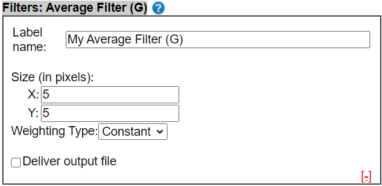
The following parameters must be specified:

Size (in pixels) – number of pixels of the moving window in pixels and lines. Values must be odd and between 1 to 21

Weighting Type – preferred weighting function; this function controls the level of spatial detail that will be preserved. The following options are available:

· Constant – a constant weighting factor of 1 is applied (default)—the least amount of spatial detail will be preserved.

· Linear – a linear weighting function is applied; the filter coefficients decrease linearly outwards from the center of the filter window

· Gaussian – a Gaussian weighting function is applied; the filter coefficients decrease according to a Gaussian function outwards from the center of the window.

Enhanced Lee Filter

The Enhanced Lee Filter was developed by Lopes in 1990. This filter not only reduces speckle noise but also preserves edge features and point targets—better than averaging filters. As a rule, larger filter windows reduce speckle levels better but also create larger spatial detail losses. It is up to the user to find a good balance between these two conflicting effects. The Enhanced Lee Filter accounts for the number of image looks (controls image smoothing) and uses a damping factor (defines the extent of exponential damping). The number of looks is read from the product metadata file.

Constraints related to this method are:

· Only non-complex or detected products can be processed. The ST includes a utility to convert complex products to detected products.

This method works for original (Level 1) input products only, i.e. CH, CV, HH, HV, VH, or VH.

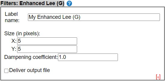
The following parameters must be specified:

Size (in pixels) – number of pixels of the moving window in pixels and lines. Values must be odd and between 1 to 21

Dampening coefficient – this parameter defines the degree of the exponential damping. A higher value increases the degree of damping and so reduces image smoothing but enhances edge preservation. A value between 0 and 1 can be entered.

GAMMA Map Filter

The GAMMA Map Filter was first proposed by Kuan in 1987 as a means to reduce SAR speckle, while preserving edges. It was later modified by Lopes to assume a Gamma-distributed image scene (previously Gaussian). Like many of the other specialized SAR speckle filters, the GAMMA Map Filter is adaptive in nature, such that the degree of smoothing is contingent on the local statistics within the filter kernel, and the size of the kernel specified. The number of looks is read from the product metadata file.

Constraints related to this method are:

· Only non-complex or detected products can be processed. The ST includes a utility to convert complex products to detected products.

This method works for original (Level 1) input products only, i.e. CH, CV, HH, HV, VH, or VH.

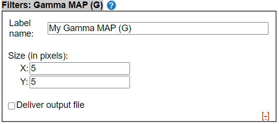
The following parameters must be specified:

Size (in pixels) – number of pixels of the moving window in pixels and lines. Values must be odd and between 1 to 21

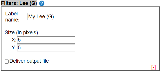
Lee Filter

The Lee Filter was developed in 1980. It was designed to reduce SAR speckle noise. Local statistics are calculated within the designated filtering kernel, with the center pixel value then replaced by the value calculated using the neighboring pixels within this window. The noise models are typically employed for the Lee filter based on the characteristics of the speckle: 1. Additive, 2. Multiplicative, and 3. Additive and Multiplicative. SAR speckle is typically multiplicative in nature. The number of looks is read from the product metadata file.

Constraints related to this method are:

· Only non-complex or detected products can be processed. The ST includes a utility to convert complex products to detected products.

This method works for original (Level 1) input products only, i.e. CH, CV, HH, HV, VH, or VH.

The following parameters must be specified:

Size (in pixels) – number of pixels of the moving window in pixels and lines. Values must be odd and between 1 to 21

Touzi-Lopes MMSE Filter

The Touzi-Lopes filter was designed as an adaptive technique to identify five specific types of features within a SAR image, and to apply speckle reduction unique to each. The objective is to achieve noise reduction while preserving point targets, curvilinear features, and edges. The filter is adaptive and controlled by changes in the coefficient of variation and the gradient of the ratio edge detector for different window sizes. The five subareas detected within the processing window include point targets, homogeneous regions, curvilinear features, edges, and isotropic areas. Following identification of a subarea type, an iterative process follows which defines the spatial extent of the feature, after which it is filtered using the appropriate kernel size and specialized filtering technique specific to the feature type. The Touzi-Lopes Filter thus removes SAR speckle while preserving attributes such as texture and fine structures. The number of looks is read from the product metadata file.

Constraints related to this method are:

· Only non-complex or detected products can be processed. The ST includes a utility to convert complex products to detected products.

This method works for original (Level 1) input products only, i.e. CH, CV, HH, HV, VH, or VH.

The following parameters must be specified:

Size (in pixels) – number of pixels of the moving window in pixels and lines. Values must be odd and between 1 to 21

Curve detection threshold – this parameter defines if a given pixel is part of a curved feature. A higher value reduces image smoothing but enhances the preservation of linear and curved features. A value between 0 and 10 must be entered—0.5 will be adequate in for most images.

Edge detection threshold – this parameters defines if a given pixel is part of an edge feature. A higher value reduces image smoothing but enhances the preservation of edge features. A value between 0 and 10 must be entered—0.5 will be adequate in for most images.

Gradient threshold – this parameter defines the variation permitted for successive windows for defining the maximum isotropic area. If a low value is entered, the size of isotropic areas is reduced. A value between 0 and 10 must be entered—0.1 will be adequate for most images.

Median Filter

The median filter operates by computing the median of all pixels values within a user-defined moving window.

Constraints related to this method are:

· Only non-complex or detected products can be processed. The ST includes a utility to convert complex products to detected products.

This method works for original (Level 1) input products only, i.e. CH, CV, HH, HV, VH, or VH.

The following parameters must be specified:

Size (in pixels) – number of pixels of the moving window in pixels and lines. Values must be odd and between 1 to 21

Utilities

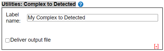
Complex to Detected Conversion

The backscatter measurements contained in Level-1 SAR products come in one of two formats, i.e. as complex numbers or as non-complex numbers. Accordingly, products that are comprised of complex numbers are commonly referred as complex products. However, products that consist of non-complex numbers are rarely referred to as non-complex products but rather as detected products. Many SAR image analysis methods only work on detected products. This routine may be used to convert complex products to a detected products and thus enable further processing by means of ‘detected only methods’.

Constraints related to this method are:

· Only complex products will be converted to detected products. However when requested to process a non-complex product, this routine will create a Warning but simply ignore the product.

This method works for original (Level 1) input products only, i.e. CH, CV, HH, HV, VH, or VH.

Incidence Angle Extraction

This routine accesses the incidence angle information available in the metadata that accompany RADARSAT-2 and RCM image products. It will compute the near-range to far-range incidence angles on the Earth ellipsoid. In other words, this routine does not account for the local topography. The output can be returned as an image raster layer or an ASCII/text array in XML format, or both.

This method works for original (Level 1) input products only, i.e. CH, CV, HH, HV, VH, or VH.

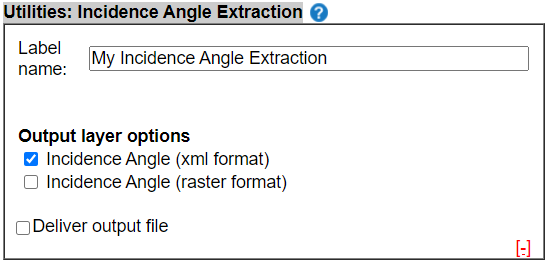
This method can generate up-to two (2) output layers.

Output layer options – Select optional output layers as desired

· Incidence Angle (XML format) (selected by default): The incidence angle information is represented in a vector format with a unique value for every pixel in range direction.

· Incidence Angle (raster format): The incidence angle information is represented in a raster format with a unique value for every pixel in range direction and repeated for every line in the image. The output consists of floating point numbers.

Polarimetry

Overview

Broadly, polarimetric decomposition methods are used to analyze backscattering behaviour by revealing different scattering mechanisms. The information obtained enhances the ability of an image analyst to spot and identify targets and to assess their physical condition. Two primary categories of decomposition methods can be identified, i.e. coherent and non-coherent decompositions. Coherent decompositions are preferred for the identification of coherent targets which are typically man-made e.g. buildings, transmission towers, ships, and aircraft. On the other hand, non-coherent decompositions are more suited for use with non-coherent targets which includes most natural surface cover types e.g. crops, forests, water, and ice cover. The EODMS SAR Toolbox includes a range of decomposition methodologies.

Freeman-Durden Decomposition

The Freeman-Durden decomposition is a non-coherent method. It operates on fully polarimetric RADARSAT-2 and RCM data by separating the covariance matrix into three distinct scattering components: surface, double-bounce, and volume scattering mechanisms. The magnitude of each scattering mechanism can be retrieved.

Constraints related to this method are:

· Complex products (SLC) are required

· Quad-polarization product are required (HH, HV, VH,VV)

This method works for original (Level 1) input products only, i.e. HH, HV, VH, and VH.

This method can generate up-to three output layers.

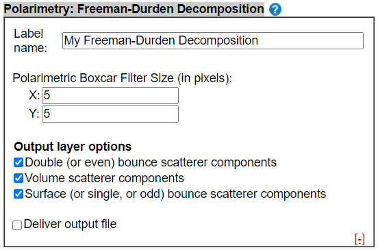
The following parameters must be specified:

Polarimetric Boxcar Filter Size (in pixels) – Enter the desired filter size in pixels (X) and lines (Y); the values entered must be odd and may range from 1 to 17.

Output layer options – Select the output layers as desired

· Double (or even) bounce scatterer components (selected by default)

· Volume scatterer components (selected by default)

· Surface (or single, or odd) bounce scatterer components (selected by default)

M-Chi Decomposition

The M-Chi decomposition is a non-coherent method and was developed specifically for the analysis of compact polarimetric SAR products such as available from RCM. This methods uses the so-called Stokes vector, the degree of polarization and the ellipticity to identify three distinct scattering mechanisms: surface, double-bounce, and volume scattering mechanisms. Only complex products that include one of two specific circular polarization combinations can be used as input, i.e. CH and CV or RR and RL.

Constraints related to this method are:

· Complex products (SLC or MLC) are required

· Compact (CH, CV) or RR, RL products are required

This method works for original (Level 1) input products only, i.e. CH, and CV.

This method can generate up to three output layers.

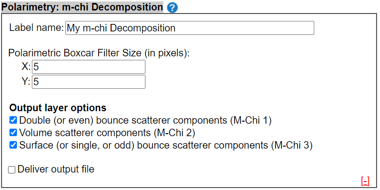
The following parameters are available:

Polarimetric Boxcar Filter Size (in pixels) – Enter the desired filter size in pixels (X) and lines (Y); the values entered must be odd and may range from 1 to 17.

Output layer options – Select the output layers as desired.

· Double (or even) bounce scatterer components (M-Chi 1) (selected by default)

· Volume scatterer components (M-Chi 2) (selected by default)

· Surface (or single, or odd) bounce scatterer components (M-Chi 3) (selected by default)

M-Delta Decomposition

The m-Delta decomposition is a non-coherent method and was developed specifically for the analysis of compact polarimetric SAR products such as available from RCM. This methods uses the so-called Stokes vector, the degree of polarization and the relative phase to identify three distinct scattering mechanisms: surface, double-bounce, and volume scattering mechanisms. Only complex products that include one of two specific circular polarization combinations can be used as input, i.e. CH and CV or RR and RL.

Constraints related to this method are:

· Complex products (SLC or MLC) are required

· Compact (CH, CV) or RR, RL products are required

This method works for original (Level 1) input products only, i.e. CH, and CV or RR and RL.

This method generates a suite of Output Layers

The following parameters must be specified:

Polarimetric Boxcar Filter Size (in pixels) – Enter the desired filter size in pixels (X) and lines (Y); the values entered must be odd and may range from 1 to 17.

Output layer options – Select the output layers as desired.

· Double (or even) bounce scatterer components (M-Delta 1) (selected by default)

· Volume scatterer components (M-Delta 2) (selected by default)

· Surface (or single, or odd) bounce scatterer components (M-Delta 3) (selected by default)

Pauli Decomposition

The Pauli Decomposition is a widely used coherent method. This approach characterises the scattering matrix as the complex sum of the matrices generated and results in representation based on the scattering characteristics of the scene being analysed. The Pauli Alpha represents the contribution of single or odd bounce scattering (sum of co-pol terms), the Pauli Beta represents the contribution of the double or even bounce returns (difference of co-pol terms) and the Pauli Gamma represents the contribution of orthogonal component or volume scattering (cross-pol term).

Constraints related to this method are:

· Complex products (SLC) are required

· Quad-polarization product are required (HH, HV, VH,VV)

This method works for original (Level 1) input products only, i.e. HH, HV, VH, and VH.

This method can generate up-to six output layers.

The following parameters are available:

Polarimetric Boxcar Filter Size (in pixels) – Enter the desired filter size in pixels (X) and lines (Y); the values entered must be odd and may range from 1 to 17.

Output layer options – Select the output layers as desired.

· Pauli Alpha: (single, or odd) bounce scatterer components – Float number (selected by default)

· Pauli Beta: (double, or even) bounce scatterer components at 0 degree – Float number (selected by default)

· Pauli Gamma: (double, or even) bounce scatterer components at 45 degrees - Float number (selected by default)

· Pauli Alpha: (single, or odd) bounce scatterer components – Complex number

· Pauli Beta: (double, or even) bounce scatterer components at 0 degree – Complex number

· Pauli Gamma: (double, or even) bounce scatterer components at 45 degrees - Complex number

Touzi Polarimetric Decomposition

The Touzi Polarimetric Decomposition is a coherent method. It operates on fully polarimetric data and produces 15 variables—in the form of images—that denote different scattering characteristics. Specifically, the orientation angle (psi), dominant eigenvalue (lambda), angle of the symmetric-scattering vector (Touzi alpha_s), vector phase difference (Touzi phi), and the helicity (Touzi tau) are computed from each one of three Eigen Vectors. The method is considered to be particularly effective for wetland classification.

Constraints related to this method are:

· Complex products (SLC) are required

· Quad-polarization product are required (HH, HV, VH,VV)

This method works for original (Level 1) input products only, i.e. HH, HV, VH, and VH.

This method can generate up-to 15 output layers.

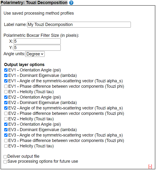
The following parameters must be specified:

Polarimetric Boxcar Filter Size (in pixels) – Enter the desired filter size in pixels (X) and lines (Y); the values entered must be odd and may range from 1 to 17.

Angle units – Select the desired units (degrees or radians) for angle-type variables.

Output layer options – Select the output layers as desired.

· EV1 – Orientation Angle (psi) (selected by default)

· EV1 – Dominant Eigenvalue (lambda) (selected by default)

· EV1 – Angle of the symmetric – scattering vector (Touzi alpha_s) (selected by default)

· EV1 – Phase difference between vector components (Touzi phi)

· EV1 – Helicity (Touzi tau)

· EV2 – Orientation Angle (psi) (selected by default)

· EV2 – Dominant Eigenvalue (lambda) (selected by default)

· EV2 – Angle of the symmetric – scattering vector (Touzi alpha_s) (selected by default)

· EV2 – Phase difference between vector components (Touzi phi)

· EV2 – Helicity (Touzi tau)

· EV3 – Orientation Angle (psi) (selected by default)

· EV3 – Dominant Eigenvalue (lambda) (selected by default)

· EV3 – Angle of the symmetric – scattering vector (Touzi alpha_s) (selected by default)

· EV3 – Phase difference between vector components (Touzi phi)

· EV3 – Helicity (Touzi tau)

Polarimetric Discriminators

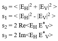
The Stokes Matrix is one example of a matrix used to describe the backscattering behaviour of the observed target. Its elements are real numbers that represent power quantities and capture both the polarized and unpolarized component of the radar return signal. The Stokes Matrix provides as a basis for the computation of a range of variables that describe the target’s backscattering behaviour.

Commonly derived variables include: the four elements of the so-called Stokes Vector, the degree of polarization, the degree of circular and linear polarization, the circular and linear polarization ratios, the relative H-V phase difference, the coherency and others. Detailed documentation for the parameters is available (Raney, 2006; Raney & al., 2011; Cloude & al., 2012; Raney & al., 2021)

Constraints related to this method are:

· Complex products (SLC or MLC) are required

· Co and cross polarized linear, circular polarization or quad-polarization product (HH and HV or VV and VH, CH and CV or HH, HV, VH and VV)

This method works for original (Level 1) input products only, i.e. CH, CV, HH, HV, VH, or VH.

This method can generate up-to 15 output layers.

The following parameters must be specified:

Polarimetric Boxcar Filter Size (in pixels) – Enter the desired filter size in pixels (X) and lines (Y); the values entered must be odd and may range from 1 to 17.

Output layer options – Select the output layers as desired.

· Stokes Vector (S0, S1, S2, S3) (selected by default)

· Degree of polarization: sqrt(s1**2 + s2**2 + s3**2)/s0 <m>

· Sine of the latitude of the Stokes vector on the Poincare sphere: sin(2*chi) = s3/(m*s0) <s2chi>

· Sine of the longitude of the Stokes vector on the Poincare sphere: sin(2*psi) = s2/sqrt(s1**2 + s2**2)) <s2psi>

· Degree of linear polarization: sqrt(s1**2 + s2**2)/s0 <m_l>

· Degree of circular polarization: s3/s0 <m_c>

· Linear polarization ratio: (s0 - s1)/(s0 + s1) 0 <= lp_ratio <lp_ratio>

· Circular polarization ratio: (s0 - s3)/(s0 + s3) 0 <= cp_ratio <cp_ratio>

· Coherency parameter |mu|: sqrt(s2**2 + s3**2)/sqrt(s0**2 - s1**2) <mu>

· Relative H and V phase difference: atan(s3/s2) (radians) <delta>

· Alpha parameter in the compact H/alpha decomposition: 0.5*atan(sqrt(s1**2 + s2**2)/s3) (radians) <alpha>

· Longitude of Stokes vector 2*psi: atan(s2/s1) (radians) <phi>

References

Charbonneau, F., (2023). Compact polarimetric equations under backward scattering alignment convention. Geomatics Canada, Open File 72, 2023, 13 pages, https://doi.org/10.4095/331496

Raney, R. K., (2006). Dual-Polarized SAR and Stokes Parameters. IEEE Geoscience and Remote Sensing Letters, Vol. 3, no. 3. pp. 317-319.

Raney, R. K. et al., (2011). The Lunar Mini-RF Radars: Hybrid Polarimetric Architecture and Initial Results, Proceedings of the IEEE, Vol. 99, no.5, pp 808-823.

Cloude, S. R, et al. (2012). Compact Decomposition Theory, IEEE Geoscience and Remote Sensing Letters, Vol. 9, no. 1. pp. 28-32, https://doi.org/10.4095/305958

Raney, R. K., Brisco, B., Dabboor, M., and Mahdianpari, M., "RADARSAT Constellation Mission’s Operational Polarimetric Modes: A User-Driven Radar Architecture", Canadian Journal of Remote Sensing, Vol. 47, no. 1, pp. 1-16, 2021. DOI: 10.1080/07038992.2021.1907566

Compact Polarization to Circular Polarization to (RR, RL)

This routine synthesizes RR and/or RL polarized images, in a detected and/or complex format, from RCM compact polarimetric (CH, CV) data products.

Constraints related to this method are:

· Compact polarization products are required (CH, CV)

· Complex products (SLC or MLC) are required

This method works for original (Level 1) input products only, i.e. CH, and CV.

This method can generate up-to four output layers.

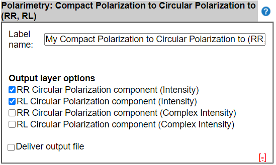
Output layer options – Select the output layers as desired.

· RR Circular Polarization component (Real number denoting Intensity) (selected by default)

· RL Circular Polarization component (Real number denoting Intensity) (selected by default)

· RR Circular Polarization component (Complex number denoting Intensity)

· RL Circular Polarization component (Complex number denoting Intensity)

Quad-Pol. to Compact-Pol. (RH, RV)

This routine synthesizes RH and/or RV polarized images, in a detected and/or complex format, from RADARSAT-2 or RCM quad-polarization (HH, HV, VH, VV) data products.

Constraints related to this method are:

· Quad polarization products are required (HH, HV, VH, VV)

· Complex products (SLC) are required

This method works for original (Level 1) input products only, i.e. HH, HV, VH, and VV.

This method can generate up-to four output layers.

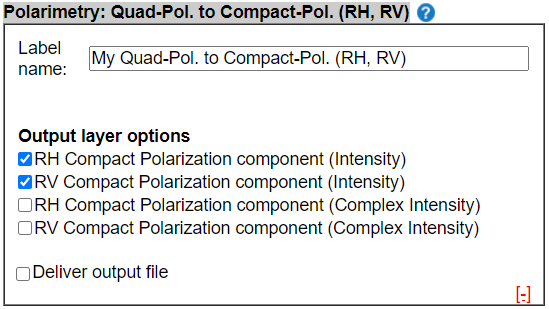
Output layer options – Select the output layers as desired.

· RH Compact Polarization component (Real number denoting Intensity) (selected by default)

· RV Compact Polarization component (Real number denoting Intensity) (selected by default)

· RH Compact Polarization component (Complex number denoting Intensity)

· RV Compact Polarization component (Complex number denoting Intensity)

Quad-Pol to Full Circular (RR, RL, LR, LL)

This routine synthesizes RR, RL, LR, and/or LL polarized images, in a detected and/or complex format, from RADARSAT-2 and RCM quad-polarization (HH, HV, VH, VV) data products.

Constraints related to this method are:

· Quad polarization products are required (HH, HV, VH, VV)

· Complex products (SLC) are required

This method works for original (Level 1) input products only, i.e. HH, HV, VH, and VH.

This method can generate up-to eight output layers.

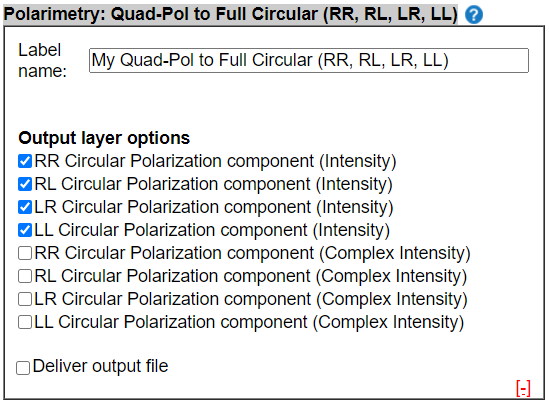
Output layer options – Select the output layers as desired

· RR Circular Polarization component (Real number denoting Intensity) (selected by default)

· RL Circular Polarization component (Real number denoting Intensity) (selected by default)

· LR Circular Polarization component (Real number denoting Intensity) (selected by default)

· LL Circular Polarization component (Real number denoting Intensity) (selected by default)

· RR Circular Polarization component (Complex number denoting Intensity )

· RL Circular Polarization component (Complex number denoting Intensity )

· LR Circular Polarization component (Complex number denoting Intensity )

· LL Circular Polarization component (Complex number denoting Intensity )

Interferometry

Overview

Interferometry describes the processes by which interferometric phase information is used to measure changes in terrain (ground deformation) between exact repeat passes of the sensor. Amplitude and phase information from single look complex (SLC ) data are used to generate standard and advanced ground deformation and change detection products. Output products are geocoded to WGS84 projection and available in GeoTIFF format with additional coarse resolution preview files in PDF and KMZ formats. Requirements for interferometric processing include exact repeat pass SLC data with overlapping geographic extents including orbital information (metadata) and an accurate digital elevation model which also overlaps with the SLC data extents. Detailed documentation for this method is available (Dudley & Samsonov, 2020; Samsonov, Feng, & Short, 2017).

Ground deformation

The ground deformation method uses Differential Interferometric Synthetic Aperture Radar (DInSAR) processing to measure small (centimeter-level) changes in the Earth’s surface between repeat passes of the sensor. Phase information is used to measure changes along the line-of-sight from the satellite to the Earth’s surface between image dates. These changes in phase can be unwrapped and converted to line-of-sight displacements. The stability of the phase measurement is quantified though its coherence. Sources of phase noise (e.g. atmospheric delays), or large surface changes can manifest as reduced coherence (decorrelation). This technique can be used for mapping ground deformation resulting from processes such as permafrost thawing, slow-moving deep-sited landslides, mining and fluids injection and extraction (oil/gas/groundwater/CO2), small earthquakes and volcanic eruptions. Coherence products can also be used to detect changes in the terrain.

Constraints to this method are:

· Only single look complex (SLC) data. Intensity and phase information are required for interferometric processing.

· Data must satisfy the exact repeat pass conditions required for interferometry. Geographic extents, orbit number, beam mode, incidence angle, polarization, and lookup table (LUT) must be the same across all data.

· The DEM must overlap geographically with the input data.

This method only accepts a single transmit/receive polarization combination (e.g. HH, VV, VH, HV, CH, or CV). Users of dual, quad, or compact polarization must identify their polarization choice. All output products are geocoded.

Processing is performed by direct coregistration using pairwise processing.

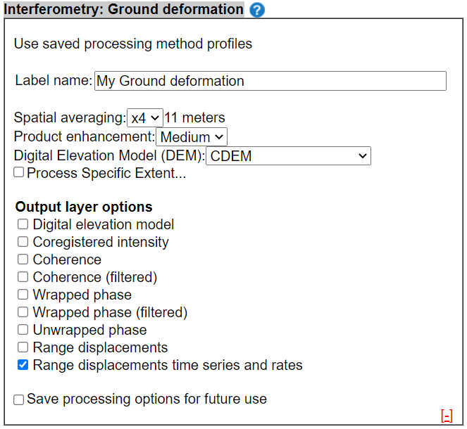
The following parameters must be specified:

Spatial averaging - Specify a value for the spatial averaging.

· Input data will be spatially multilooked (averaged) by this factor to improve coherence.

· For user information, the approximate spatial resolution of the output products is displayed in meters.

Product enhancement - Specify a level for the product enhancement.

· Additional adaptive spatial filtering, coherence thresholds, and interpolation and regularization of time series results are modified by this parameter.

· A higher level increases the adaptive spatial filtering, interpolation, and regularization strengths and raises coherence thresholds. The available levels are: Low, Medium, and High.

Digital Elevation Model (DEM) - Select the preferred DEM for processing.

· CDEM (Canada at 20m resolution)

· CDSM (CDEM+SRTM, Canada south of 60°N at 20m resolution)

· SRTM 30m (Canada south of 60°N at 30m resolution)

· SRTM 90m (World between 56°S and 60°N at 90m resolution)

· SRTM 30m (World between 56°S and 60°N at 30m resolution)

· ASTER 30m (World at 30m resolution)

Process Specific Extent – Specify a sub-region for processing (optional).

· Use current map extent.

· Draw an area (rectangle or polygon). Polygons will be modified to a rectangular bounding box during processing.

· Enter coordinates.

Output layer options – Select the desired output layers.

· Digital elevation model – Coregistered digital elevation model for each image date.

· Coregistered intensity – Coregistered intensity product for each image date.

· Coherence – Coregistered interferometric coherence for each date pair.

· Coherence (filtered) – Coregistered interferometric coherence for each date pair after adaptive spatial filtering.

· Wrapped phase – Coregistered interferometric wrapped phase for each date pair.

· Wrapped phase (filtered) – Coregistered interferometric wrapped phase for each date pair after adaptive spatial filtering.

· Unwrapped phase – Coregistered interferometric unwrapped phase for each date pair after adaptive spatial filtering and phase unwrapping.

· Range displacement (selected by default) – Coregistered range displacement for each date pair after conversion from unwrapped phase to line-of-sight displacement.

· Range displacement time series and rate (selected by default) – Cumulative line-of-sight displacement for all image dates including the linear displacement rate.

Very large ground deformation

The Very large ground deformation method uses Speckle Offset Tracking (SPO) to measure large changes (meter-level) in the Earth’s surface between exact repeat passes of the sensor. Using both phase and intensity information, image patches are cross-correlated and shifts in pixel locations between image dates can be measured along both azimuth and range directions. Comparing these correlations to other nearby correlations yields a signal-to-noise statistic which is used as a measure of quality. If the measured ground movement is known to follow local terrain gradients (surface parallel flow), then the ground movement can be derived in the east/west, north/south, and up/down directions. This technique can be used for mapping glacier ice flow, fast moving deep-sited landslides, and large earthquakes and volcanic eruptions.

Constraints to this method are:

· Only single look complex (SLC) data. Intensity and phase information are required for offset tracking processing.

· The DEM must overlap geographically with the input data.

Processing is performed by direct coregistration using pairwise processing.

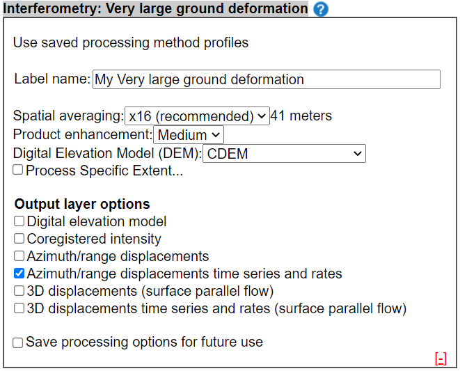
The following parameters must be specified:

Spatial averaging - Specify a value for the spatial averaging.

· Input data will be spatially resampled by this factor.

· For user information, the approximate spatial resolution of the output products is displayed in meters.

Product enhancement - Specify a level for the product enhancement.

· Additional adaptive spatial filtering, coherence thresholds, and interpolation and regularization of time series results are modified by this parameter.

· A higher level increases the adaptive spatial filtering, interpolation, and regularization strengths and raises coherence thresholds. The available levels are: Low, Medium, and High.

Digital Elevation Model (DEM) - Select the preferred DEM for processing.

· CDEM (Canada at 20m resolution)

· CDSM (CDEM+SRTM, Canada south of 60°N at 20m resolution)

· SRTM 30m (Canada south of 60°N at 30m resolution)

· SRTM 90m (World between 56°S and 60°N at 90m resolution)

· SRTM 30m (World between 56°S and 60°N at 30m resolution)

· ASTER 30m (World at 30m resolution)

Process Specific Extent – Specify a sub-region for processing.

· Use current map extent.

· Draw an area (rectangle or polygon). Polygons will be modified to a rectangular bounding box during processing.

· Enter coordinates.

Output layer options – Select the desired output layers

· Digital elevation model – Coregistered digital elevation model for each image date.

· Coregistered intensity – Coregistered intensity product for each image date.

· Azimuth/range displacements – Coregistered displacements in the range and azimuth directions for each date pair.

· Azimuth/rage displacements time series and rates (selected by default) – Cumulative azimuth and range displacements for all image dates including the linear displacement rates.

· 3D displacements (surface parallel flow) – Coregistered displacements in the east/west, north/south, and up/down directions for each date pair assuming surface parallel flow constraint.

· 3D displacements time series and rates – Cumulative east/west, north/south, and up/down displacements for all image dates including the linear displacement rates assuming surface parallel flow constraint.

References

Dudley, J., & Samsonov, S. (2020). The Government of Canada automated processing system for change detection and ground deformation analysis from RADARSAT-2 and RADARSAT Constellation Mission Synthetic Aperture Radar data: description and user guide. Natural Resources Canada. Geomatics Canada, Open File 63. https://doi.org/10.4095/327790

Samsonov, S., Feng, W., & Short, N. (2017). DInSAR products and applications for the RADARSAT Constellation Mission. Natural Resources Canada. Geomatics Canada, Open File 37. https://doi.org/10.4095/305958

EODMS SAR Toolbox Processing Product Order Delivery Format Definition

EODMS SAR Toolbox Processing Order Universal Unique Identifier (UUID)

All EODMS SAR Toolbox (ST) processing orders are identified through a distinct Universal Unique Identifier (UUID). All files (products, output layers, and metadata) corresponding to a specific processing request comprise the same UUID within their metadata. As such, the processing history of each product and the origin of all resulting output layers is known. The UUID is either provided as part of a filename or as a metadata tag within a product or output layer. The metadata tags in products and output layers can be accessed with the “gdalinfo” utility available in the Geospatial Data Abstraction Library (GDAL) suite of programs (https://gdal.org/index.html ). GDAL works in all environments and is Open Source.

A Universal Unique Identifier (UUID) looks like this: 17ce4b53-5157-43ea-ba1e-7464e471d7e1.

The EODMS ST team will ask you to provide the UUID of your processing order in the event you seek its support for one of your processing requests.

Note that the information in the following sections does not apply to the Interferometry methods (Ground deformation and Very large ground deformation) which maintain unique folder structures and file naming conventions. For Interferometric methods and delivery directory structure and files, please refers to https://doi.org/10.4095/327790

SAR Toolbox Order Metadata file

The work order metadata file provides a record of all parameters which were selected in building the SAR Toolbox work order through the EODMS system. This includes information related to how the products were processed, default values for unspecified parameters, and possible warnings related to some methods. The Directory Structure Map, presented in the following section, provides a complete diagram of the output products and directory structures created by the request.

The naming convention of the ST work order metadata file is as follows: “eodms_st_order_<UUID>.xml”.

The SAR Toolbox Order metadata file can be divided in 2 sections. The first section relates to the definition of the processing request (XML tag <processingRequest>) and comprises information about the selected: products, methods, parameters, and output layers. In essence, all decisions made by the user while defining a processing request are captured in sequence in this section. In addition, the processing order name, submission date, and the name and email address of the user are recorded. The second section relates to the execution of the processing request, i.e. the product generation (XML tag “<productGeneration>”) and comprises information about: applied processing methods, user specified parameters, ST defaulted/assumed parameters, and ST issued Warning and Readme messages. This section also records the following for each input product and output layer: filename, format, location relative to the UUID root directory, a description, and file attributes including size in pixel/lines, data type, product units and bits per pixel.

Directory Structure Map file

The EODMS ST generates a directory structure map file in three different formats (i.e. HTML, acsii/text and XML). These utility files define the directory structure of the processing order. The HTML and text file help to visualise the directory structure, while the XML file facilitates the programmatic extraction of file locations. Note that the information contained in the directory structure map file can also be found in the SAR Toolbox order metadata file.

The naming convention of the ST directory structure map files is as follows:

eodms_st_directories_<UUID>.html

eodms_st_directories_<UUID>.txt

eodms_st_directories_<UUID>.xml

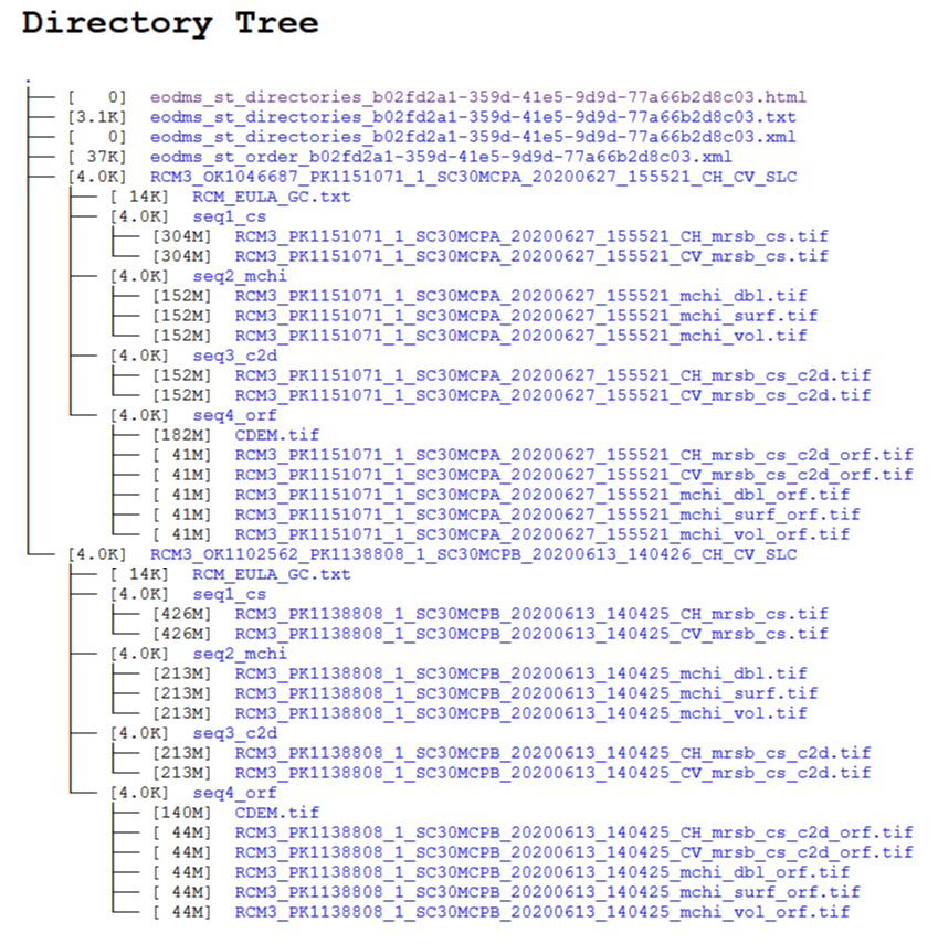
The Figure above shows an example of a directory structure map file in the html format.

Directory Structure

The name of the root directory matches the Universal Unique Identifier (UUID) of the processing request. This directory contains the ST Order Metadata file, the Directory Structure Map file in three different formats, and a series of sub-directories, i.e. one for each input product selected for processing. The names of these sub-directories—also known as product folders—match the original RADARSAT-2 or RCM product order keys.

Each product folder contains the associated End-User Licence Agreement and a series of sub-directories—also known as processing sequence folder(s). These folders are named as follows: seq<seq_id>_<processing_method>. The <seq_id> is an integer number that indicates the rank of the processing method in the overall processing sequence, i.e. the sequence identifier as defined by the user at step 3 when defining the processing order sequence. The abbreviations of the available processing methods are explained in the figure of the “Suffix” section.

Finally, each processing sequence folder contains the requested image products and/or output layers—also known as output products. The folder associated with the method that completes the overall processing sequence will always contain output product files—even if none were selected by the user. In contrast, folders associated with preceding methods will only contain output product files if they were specifically requested by the user. In other words, the user can choose to opt-out of the delivery of intermediate output products.

Image product and Output layer naming convention

The names of output products delivered by the EODMS SAR Toolbox comprise two parts:

1) an unique prefix which derives from the original product order key, and

2) a suffix which captures information about the selected sequence of processing methods, output layers, and, in some instances, the polarization of the input product.

Prefix

The prefix for output products that were generated from RADARSAT Constellation Mission (RCM) acquisitions contains the following elements:

RCM<SatelliteId>_ PK<ProductId>_<Beam>_<Date>_<Time>_

Where:

<SatelliteId> indicates the satellite number (i.e. 1, 2 or 3)

<ProductId> is composed of <Production Request ID>_<Product Sequence ID>

<Beam> indicates the beam mode

<Date> indicates the acquisition date

<Time> indicates the acquisition time

For example, the prefix for an output product created from a RCM acquisition with product order key “RCM2_OK1070060_PK1093136_2_SC30MCPC_20200505_110336_CH_CV_SLC” would be “RCM2_PK1093136_2_ SC30MCPC_20200505_110336_”.

The prefix for output products that were generated from RADARSAT-2 acquisitions contains the following elements:

RS2_ DK<DeliveryId>_<Beam>_<Date>_<Time>_

Where:

<DeliveryId> corresponds to the Delivery ID

<Beam> indicates the beam mode

<Date> indicates the acquisition date

<Time> indicates the acquisition time

For example, the prefix for an output product created from a RADARSAT-2 with product order key “RS2_OK111018_PK988914_DK927637_U22_20190908_141558_HH_SLC” would be “RS2_DK927637_ U22_20190908_141558_”.

Suffix

The suffix for output products is independent of the satellite source and contains the following elements:

<Input_Polarization>_<Method_Abbreviation>_<Output_Layer>

Where:

<Input_Polarization> indicates the polarization of the input product; where applicable only e.g. for radiometric calibration and speckle filtering.

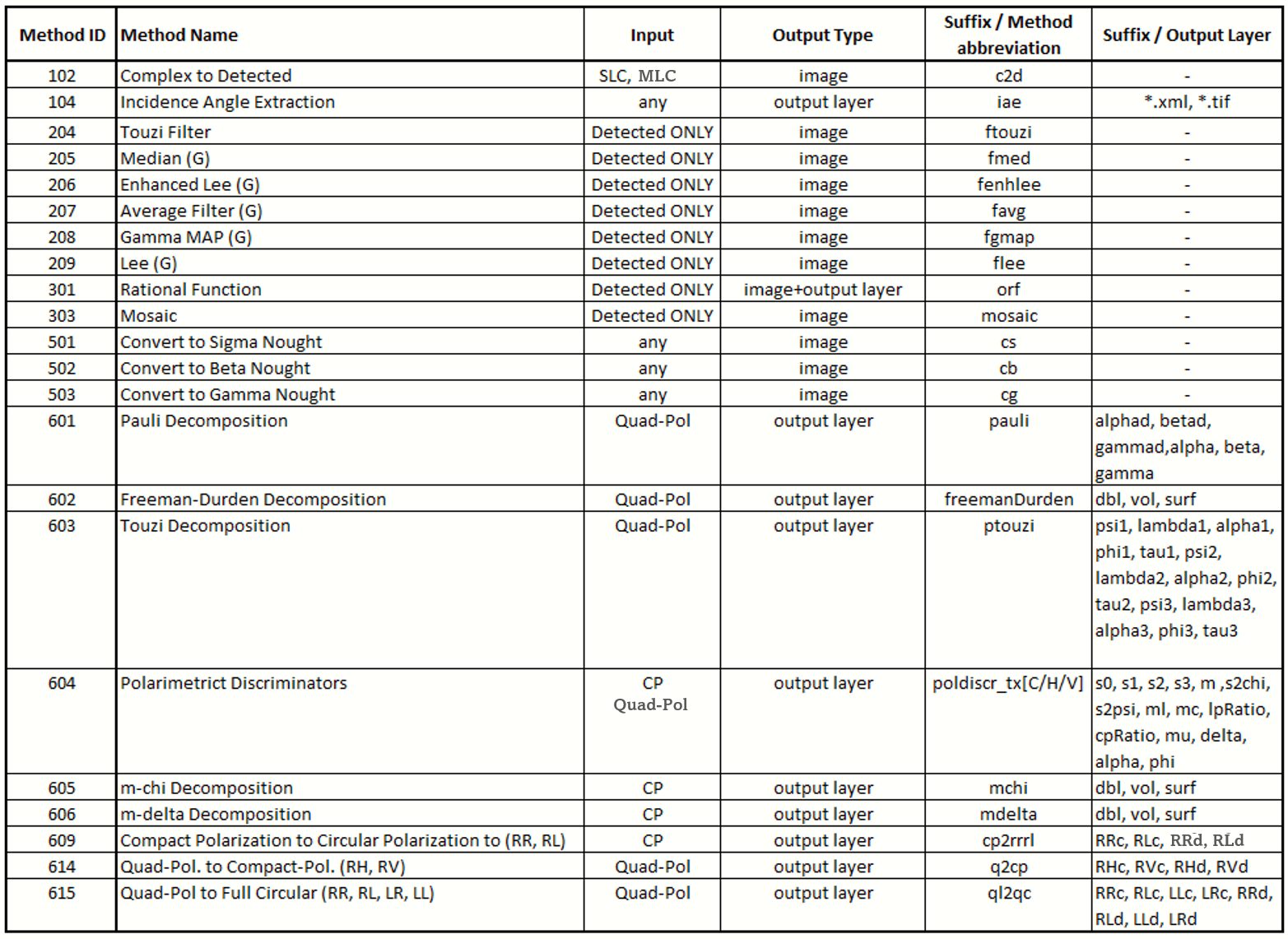
< Method_Abbreviation> indicates the abbreviation of the processing method applied (column 5 in figure below)

< Output_Layer> indicates the abbreviation of the output layer as selected by the user; where applicable only e.g. for polarimetric decompositions, ground deformation, and lake ice extent (column 6 in figure below).

The figure below defines all currently available method abbreviations and, where applicable, the optional output layers.

For example, the suffix for the Double Bounce output product created by the M-Chi decomposition would be “mchi_dbl”.

In Summary: Directory + Prefix + Suffix

Assume the following input product, processing method, and output layer were selected by the user:

· Input product file; RCM acquisition with product order key “RCM1_OK1222952_PK1262635_2_5MCP17_20200920_022723_CH_CV_SLC”.

· Processing method; M-Chi Decomposition—ranked 3^rd in the overall processing sequence.

· Output layer; Double (or even) bounce scatterer components.

Accordingly, output directory and output product would be named as follows:

· Directory: <UUID>/RCM1_OK1222952_PK1262635_2_5MCP17_20200920_022723_CH_CV_SLC/seq3_mchi/

· Product: RCM1_ PK1262635_2_5MCP17_20200920_022723_mchi_dbl.tif

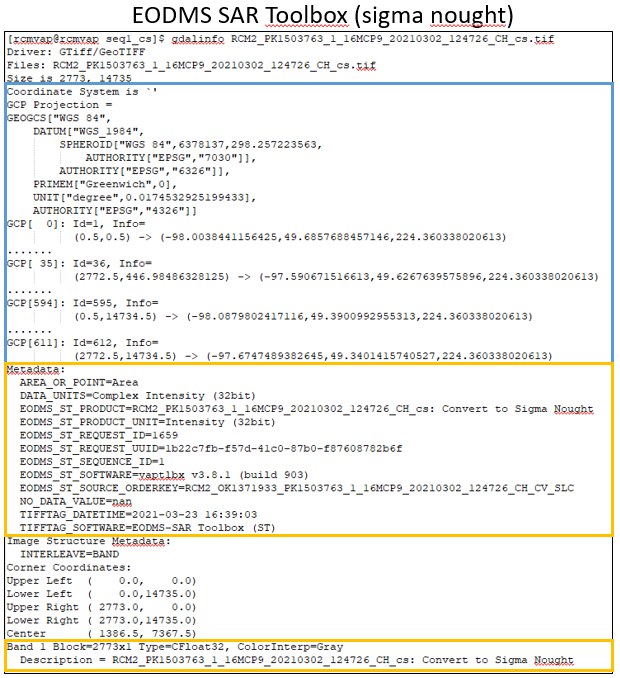
Metadata within the Geotiff product

As a rule, the raster output files produced by the ST include the same georeferencing information and ground control points (GCPs) as the Radarsat-22 or RCM original input product file. The output files created by the Ortho-rectification (Rational Function) and Mosaic methods deviate from this general rule.

Below is an example of a report created with the “gdalinfo” utility available in the Geospatial Data Abstraction Library (GDAL) suite of programs (https://gdal.org/index.html ). The section marked by the blue frame comprises the georeferencing information and the GCPs. The sections outlined in orange contain the EODMS SAR Toolbox metadata tags including the UUID of the processing request and sequence identifier of the processing method (convert to sigma nought, cs abbreviated).